How to Create a Work Order Tracker using Pivot Tables in Google Sheets

The ability to track work orders efficiently can make a significant difference in any business, whether you’re managing a small team or running a larger operation. A work order tracker helps you keep tabs on tasks, deadlines, and resources, making your life easier and your projects more manageable. Google Sheets is a fantastic tool for this, especially with the features of pivot tables.

What Is a Pivot Table?

A pivot table is a handy tool that helps you quickly organize and summarize data in Google Sheets. It lets you sort, count, or total up your data without changing the original information.

Think of it as a way to rearrange your data to spot patterns and get insights easily. This makes pivot tables a go-to feature for anyone who needs to analyze large amounts of data and make smart decisions based on what they find.

Step 1: Set Up Your Data

First, create a new Google Sheet and list the key columns like:

• Work Order ID
• Date
• Task Description
• Assigned Person
• Priority (Low, Medium, High)
• Status (Open, In Progress, Closed)

Make sure every row is a new entry and each column has a clear label.

Step 2: Enter Information

Gather the information you need to track in your work order system.

Step 3: Use Dropdown Menu

Use the dropdown menu for recurring information, such as Priority and Status. To do this, select the cells where you want to put your dropdown menu and click Insert > Dropdown. Then, enter the options you want to use. In this example, I’ll add High, Low, and Medium as the Priority options.

Step 4: Insert a Pivot Table

Select the entire data range you want to analyze. You can do this by clicking and dragging over your data or pressing Ctrl+A on your keyboard.

Once your data is selected, go to the top menu and click Insert. From the dropdown, select Pivot Table. Choose whether to place the Pivot Table in a new or similar sheet, then click Create.

Step 5: Add Rows and Columns

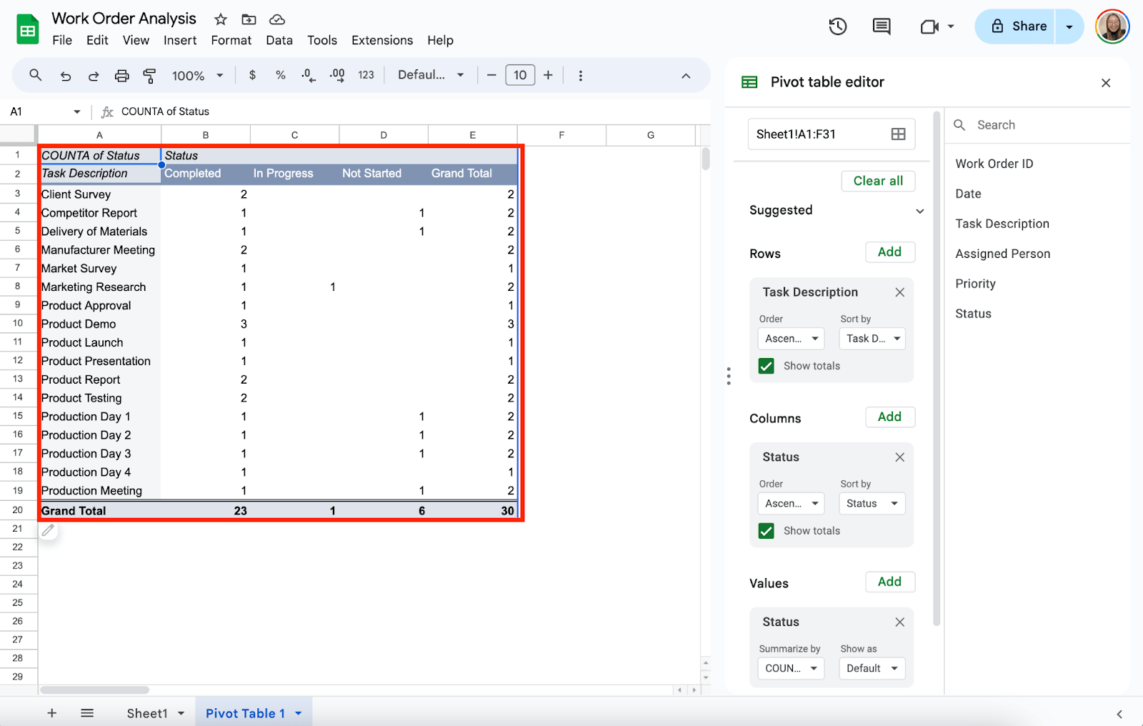
Now you’ll start building your Pivot Table. A Pivot Table editor will appear on your screen’s right side. Click “Add” beside “Rows” and choose the column you want to appear as rows. For example, you might select Task Description to see who is responsible for each work order.

Under Columns, you can add another dimension. For example, you could add Status to see a breakdown of work order status.

Step 5: Fill in the Values

Next, you’ll want to add some data to the table. Under Values, click Add and choose something you want to summarize, like Status.

Get the Free Work Order Template

Get a copy of the free Work Order Template. I’ve populated some cells as example but you can customize them as needed.

Final Thoughts

Using Pivot Tables in Google Sheets is a great way to manage and keep track of work orders. It helps you quickly see which tasks need attention, who’s responsible for them, and their priority—all in one clear, organized view.

Frequently Asked Questions

Is it possible to filter work orders in the Pivot Table by date?

Add the Date column to the Filters section in the Pivot Table editor. This allows you to view only the work orders from specific periods, which is especially useful when managing weekly or monthly tasks.

How can I track the total work orders using a Pivot Table?

Add the Work Order ID column to the Values section of the Pivot Table editor to track the total number of work orders. Google Sheets will automatically count the entries, showing you the total work orders in your system.

Can I track multiple work orders across different sheets using a Pivot Table?

If your work orders are spread across multiple sheets, you can consolidate them into one Pivot Table by importing data from each sheet using Google Sheets’ IMPORTRANGE function. This allows you to create a unified Pivot Table that tracks work orders from different sources.