How to Create a Monthly Net Worth Tracker Using Charts in Google Sheets

Do you want to get a clear snapshot of your financial health? Tracking your net worth monthly can help you see where you stand, what you own (your assets) and what you owe (your liabilities). One effective and interactive way to do this is using charts in Google Sheets.

What Is a Net Worth?

Your net worth is like a snapshot of your financial health, showing the difference between what you own (assets) and what you owe (liabilities). Assets include cash, investments, property, and anything else of value, while liabilities cover debts like loans and credit card balances.

A positive net worth indicates that your assets exceed your liabilities, suggesting financial stability and greater freedom. In contrast, a negative net worth means you owe more than you own, pointing to areas needing improvement.

Step 1: Open a New Google Sheet

Start by opening Google Sheets and creating a new blank spreadsheet. You can name it “Net Worth Tracker” to stay organized.

Step 2: Set Up Your Tables and Categories

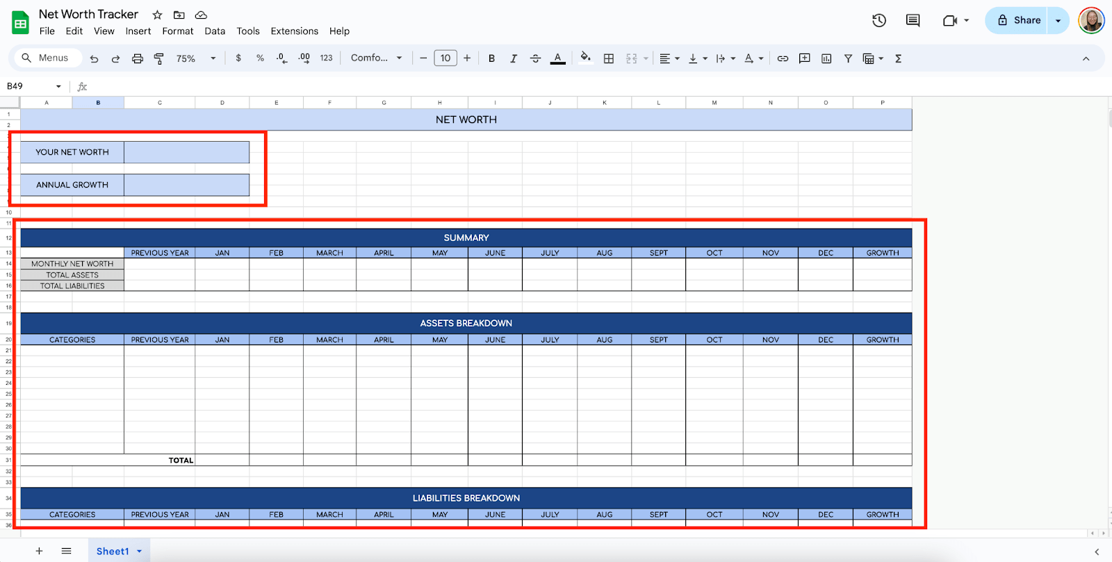
In the first rows, list your net worth computation tables and main categories. You can include labels like:

• Net Worth
• Annual Growth
• Assets
• Liabilities

You may also want to leave spaces for the charts.

Step 3: Enter Your Subcategories

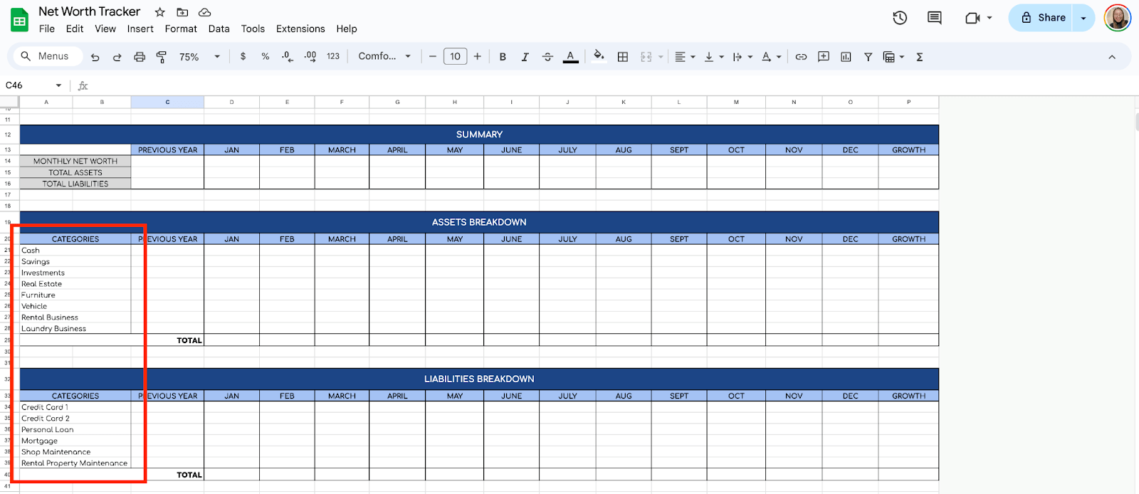
Now that your Assets and Liabilities tables are all set, it’s time to list down the subcategories for each. Here are some of the most commonly used subcategories for Assets and Liabilities:

• Assets
  • Cash
  • Savings
  • Investments
  • Real Estate
  • Furniture
  • Vehicle
  • Business
• Liabilities
  • Credit Card Debt
  • Loans
  • Mortgage
  • Business Maintenance

Leave space for additional categories you may want to add later.

Step 4: Input Your Assets and Liabilities

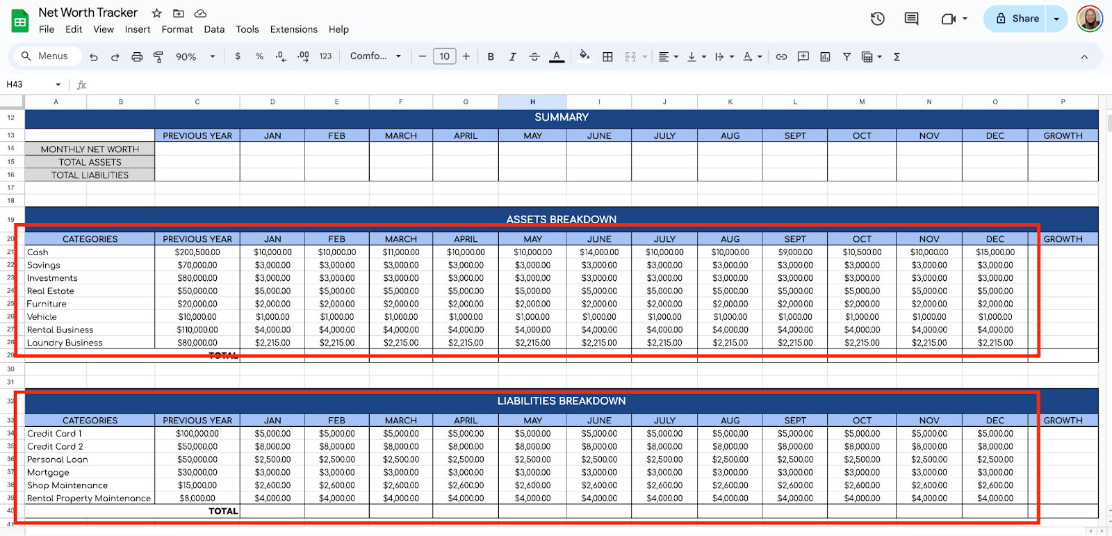
Input the values for each of your assets and liabilities. Each month, fill in the amounts for each category.

Step 5: Calculate Total Assets and Liabilities

In a new row, calculate the total assets. Do this by summing all the asset values for each month. For example, use the formula:

=SUM(D21:D28)

Do the same calculation for the rest of the months.

Next, Liabilities table, calculate the total liabilities using a similar formula for your liability categories:

=SUM(D34:D39)

Step 6: Add a Grand Total Fields

Add another row for the grand total of your entire year’s Assets and Liabilities. Use =SUM(D29:O29). Do the same for the Liabilities table.

Step 7: Calculate Net Worth

In Summary table, create a formula to calculate your monthly net worth by subtracting your total liabilities from your total assets. Use this simple formula:

=D29-D41

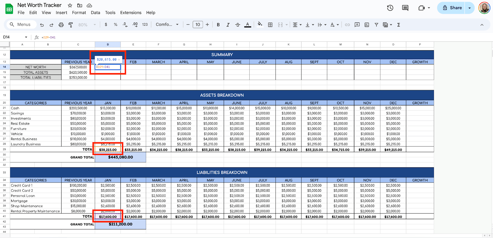
Copy this formula down the entire column to calculate your net worth for each month.

Now, for the Total Assets and Total Liabilities field on the Summary table, use the formula:

=SUM(D21:D28)

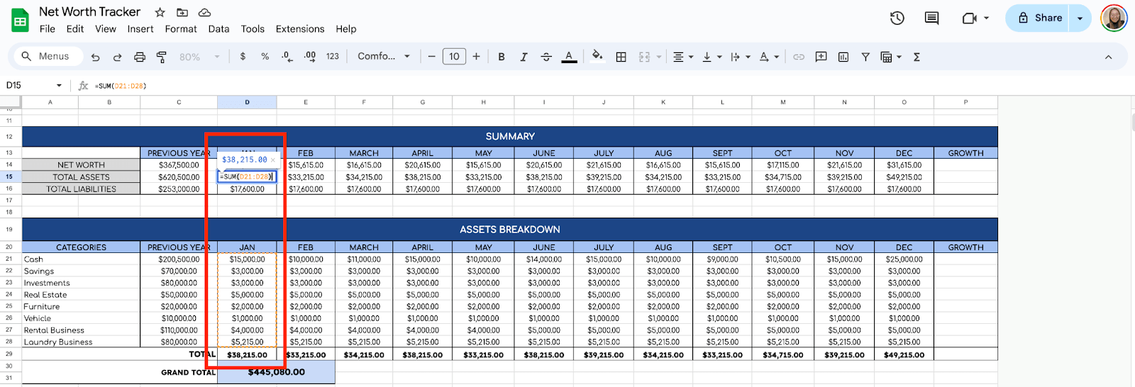
Then, scroll up to the Your Net Worth field at the top of your spreadsheet and calculate your total Net Worth for the year. Use the formula:

=SUM(D14:O14)

For the Annual Growth, use the formula:

=C14-C4

Step 8: Create Charts for Visualization

Now that you have all the necessary data, it’s time to create charts to visualize your net worth over time.

Let’s work on the Net Worth chart first. To use charts, highlight the months and the net worth values. Click “Insert” in the top menu, then select “Chart.” Google Sheets will automatically generate a chart.

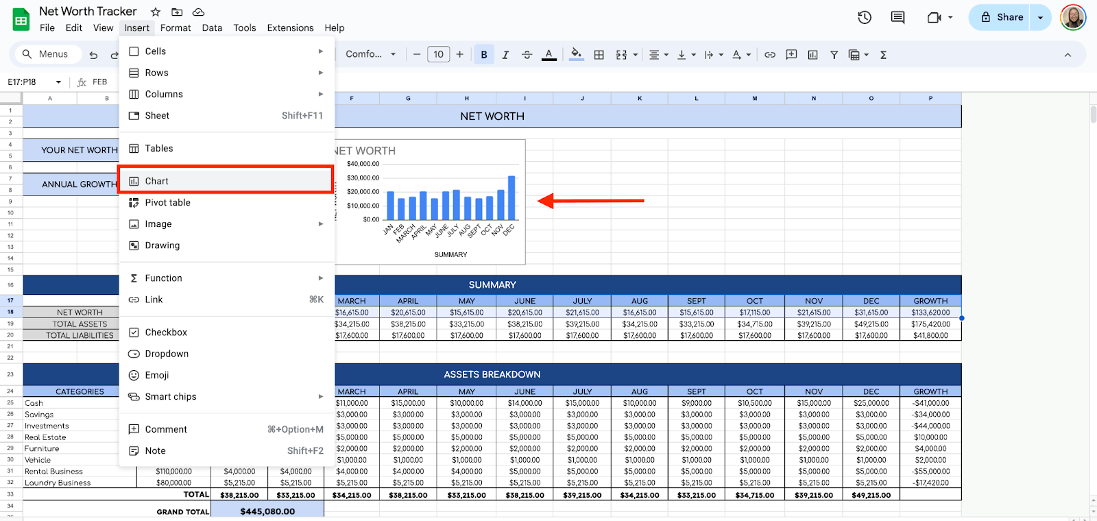
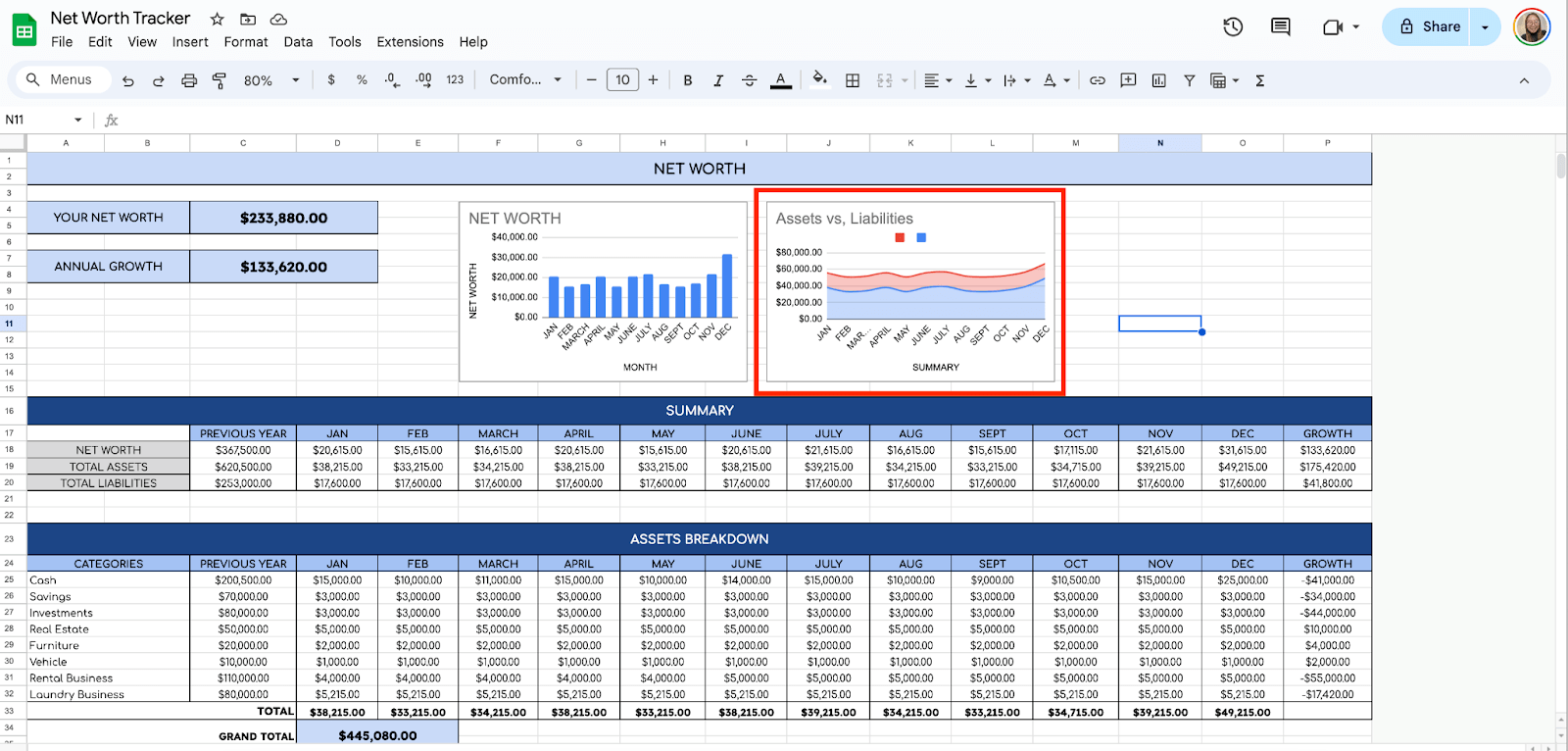
Change the chart type to a line chart for better tracking over time. Adjust the chart title and axis labels to make the chart easy to read. For example, label the chart “Net Worth” and ensure the X-axis shows the months while the Y-axis shows the net worth. Do the same steps to get the visual presentation for the Assets vs. Liabilities chart.

Result:

Asset vs. Liabilities Chart

Step 9: Customize the Chart

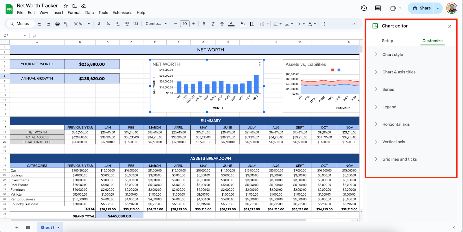
You can customize your chart by clicking on it and selecting “Chart Editor” on the right. You can change colors to make the chart visually appealing, adjust line thickness, and add data labels to show the exact net worth figures.

Get the Free Monthly Net Worth Tracker

Get a copy of the free Monthly Net Worth Tracker. I’ve populated some cells as examples, but you can customize them as needed.

Final Thoughts

Personally, I’ve found that visualizing it with charts makes a big difference in staying motivated. I mean, seeing that line go up over time? That’s satisfying. And honestly, don’t overcomplicate it. Keep it simple, be consistent with updates, and let the data guide your financial decisions. The peace of mind that comes with knowing where you stand is worth the effort.

Frequently Asked Questions

Can I automatically update my assets and liabilities, like stocks & mutual funds, in Google Sheets?

You can use functions like GOOGLEFINANCE to track assets like stocks or mutual funds in real time. Manual updates are necessary for most other categories unless you use third-party add-ons or scripts.

What happens if I delete a month’s data accidentally?

Google Sheets has a ‘Version history’ feature. You can access it by going to “File” > “Version history” > “See version history,” where you can restore your sheet to a previous state.

Can I protect my Google Sheet to prevent accidental changes?

Yes, you can protect specific sheets or ranges to avoid accidental edits. Highlight the cells or ranges you want to protect. Right-click and select “Protect range.” You can then set permissions for who can edit those cells, ensuring the integrity of your formulas and data.