
Do you plan a tournament and wish your spreadsheet could highlight important details automatically? Conditional formatting in Google Sheets can do just that!
It’s a simple yet useful feature that makes your tournament data more organized and easier to read. Regardless if you want to highlight winners, mark certain scores, or track progress through different rounds, conditional formatting allows you to set up rules that make your spreadsheet visually engaging and efficient.
Why Are Tournament Records Important?
Tracking tournament records with a spreadsheet is a great way to stay organized and avoid confusion. It helps you easily see each team’s or player’s performance, track wins, losses, and rankings, and make strategic decisions. Plus, it simplifies post-event reporting and future planning, ensuring everything runs smoothly for both participants and organizers.
Step 1: Set Up the Spreadsheet
Start by opening a new spreadsheet in Google Sheets, then click “+ Blank” to create a new sheet. At the top of the sheet, name your tournament. For example, “2024 Sports Tournament.” This will help you and others quickly recognize what the spreadsheet is for.
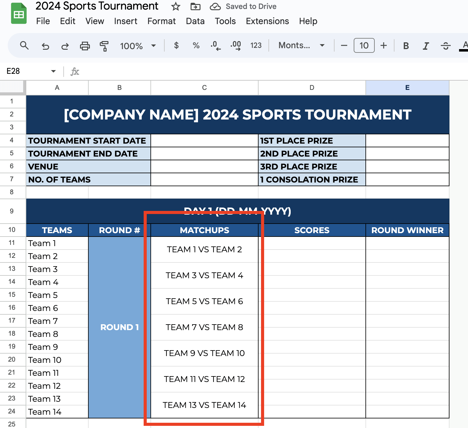
Then, create your header, where all the tournament basic information can be found.

Step 2: List the Teams or Players
In the first column, list the teams or players that will be participating. Start from cell A10 and go downwards, filling in the names.

If it’s a large tournament, add more rows for additional teams or players.
Step 3: Create a Match Schedule
Now, move to the Matchups column. This is where you can start listing the matchups.
Step 4: Add a Score Column
Next, we’ll need a place to track scores. In the next column (D), label it “Scores.” Underneath that, as the tournament progresses, you’ll enter the scores for each game.

Step 5: Calculate the Winner of Each Round
You can use a formula to determine the winner of each match automatically. Let’s say you want the winner’s name to appear in the next column (E). You can write a simple “IF” formula like this:
=IF(E11 > E12, A11, A12)
This formula checks which team has the higher score in column D. If the first team has a higher score, the formula will display the name of the first team. Otherwise, it will show the name of the second team.

Step 6: Highlight the Champions
Once all rounds are finished, you’ll have your final matchup and winner. Celebrate the champion by adding some fun formatting to their name. You can change the font color, bold it, or even use conditional formatting to make it stand out.
To use Conditional Formatting, select the Scores column and click on Format in the top menu. Choose Conditional Formatting, then click “Format cells if.” You can set rules based on what’s in the cells. Choose “Custom formula Is” for conditional formatting.
=E11>E12
Set your desired formatting style, then click Done. Now, whenever the value in E11 is greater, E11 will be highlighted, and when the value in E12 is greater, E12 will be highlighted. You can set this rule to the rest of your Scores cells.

Step 7: Track Tournament Progress
Add a new table for each round if needed to keep everything clear. For example, once Day 1 is done, create a new table in the spreadsheet and label it “Day 2.”
In the new table, list the winners of Round 1 like you did, and then create new matchups for the next round.

You can easily share your tournament spreadsheet with participants or others who might be interested. Click on the “Share” button in the top right corner and either send it via email or create a shareable link.

Get the Free Tournament Template
Get a copy of the free Tournament Template. I’ve populated some cells as examples, but you can customize them.
Final Thoughts
When setting up a tournament in Google Sheets, I find it’s best to keep things flexible and not overthink it. The tools are there to help, but they don’t need to be intimidating. Instead of aiming for perfection, focus on staying organized and making it fun. As I play around with features like conditional formatting, I always find new ways to make the sheet work better for me.
Frequently Asked Questions
How can I calculate rankings or standings in a league-style tournament?
If your tournament is based on points or rankings (rather than elimination), you can calculate standings using the SUM and RANK formulas. To sum points for each team across multiple rounds, use: =SUM(C2:F2). To rank teams by their total points, use: =RANK(G2, $G$2:$G$10)
Can I create a chart or visual representation of the tournament in Google Sheets?
Yes, you can create visual charts by using Shapes (found in the Insert menu) to draw a bracket or other visual structures or using Google Sheets’ Chart feature to track team performance over time (for league-style tournaments).
How can I protect certain cells in the spreadsheet, like the match schedule or formula cells?
To protect important cells (like formulas or matchups), you can select the cells you want to protect. Right-click and choose Protect range. Set permissions so that only you or selected users can edit those cells. This will prevent accidental changes to key parts of your tournament tracker.
The Bottom Line:
One keeps you awake. The other gets work done.
A month of coffee: $80
A month of FileDrop: $19
Why not have both?

